Full table scan burning CPU

This post is not so much a serious investigation, rather, a few curious observations, followed by some general musings prompted by them.

So… When you see a SQL execution plan and runtime statistics like below, what thoughts come to mind?

Some fairly obvious observations are that this is a full table scan, it’s taking place on an Exadata system (“STORAGE” keyword in “TABLE ACCESS STORAGE FULL” should tip you off about that), and it’s taking a long time to run. Why is it so slow?

Of course, it’s a full table scan, and almost everyone in the database world knows that full scans are slow. But on the other hand, it’s an Exadata. Aren’t full scans supposed to be fast on Exadata? And even if they are slow, certainly not this slow (152 seconds to read meagre 212MB bytes and do 28k logical reads?). Aren’t full scans in Exadata supposed to be “smart”?

Someone more observant and with a bit of background in Exadata performance tuning might also note that the smart scan is not happening here: cell multi block physical read wait event tells us that much. TABLE ACCESS STORAGE FULL was telling us otherwise, but that was what the optimiser was thinking, and the wait events are telling what was actually happening.

But OK, even without all those Exadata smart bells and whistles, this slowness is kinda extreme. Most of us have hard drives at home that would read that much data in a couple of seconds (if not a fraction of a second). So what’s happening?

Another telling sign is that 99% of time is spent on CPU. So data transfer speed clearly isn’t an issue here. However, this SQL didn’t look like your typical CPU-intensive query: it was merely selecting 5 columns without transforming from a single table with a long in-list in a WHERE section, once again, without any subqueries or transformations, just a bunch of bind variables. Parsing would be certainly a suspect for anything with a long in-list, but it was checked and ruled out (by looking at ASH’s in_parse column and other relevant diagnostics).

At this point I took a stack profiling sample (as usual, using orafun.info for function name lookup). Since the flame graph had a more or less rectangular shape (i.e. most of the time spent in a single branch), this is the code path of interest:

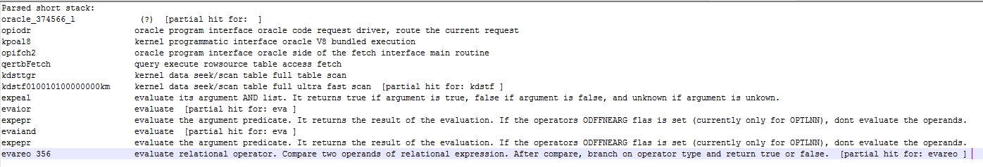
Now we have it: the time is spent evaluating the predicates. Yes, they didn’t contain any complex expressions, but that long in-list.. well, it was really, really long, almost a 1,000 pairs of numbers. The table being full scanned contained 100M rows. According to the execution plan, only 113K out of them would be returned by the query, but before that happens, all 10M rows need to be checked if they match the condition in the WHERE clause… which means 20 billion comparisons! Modern CPUs are supposed to be good at comparing numbers fast, but 10 ns doesn’t sound crazy (although it probably has more to do with the CPU cache access latency than any actual CPU cycles spent calculating).

Fixing the problem isn’t a particularly interesting part, although it probably depends on how exactly one defines “fixing”. If the only goal is to improve performance of the query in question, that’s relatively straightforward — all you need to do is nudge the optimiser to use an index, and this this particular case it was sufficient to gather optimiser stats to achieve that (it would be also interesting to investigate why the estimates based on dynamic sampling are off by that much, but I didn’t really have time for that). On the other hand, perhaps a more relevant question is: how did this query come about? What is it trying to achieve?

Often, such queries are a part of some batch loading framework written in Java or some other language. Programmers like to use such coding patterns for several reasons:

1. Control (you know how many batches you loaded, so you can keep track of the progress)
2. Resilience and performance (so you can commit each small batch preventing loss of progress if it fails half-way)
3. Code reuse (when you have such framework for copying one kind of data, it’s tempting to extend it to use with other kinds of data as well).
   

These reasons may have been justified to some extent in the past, but nowadays this approach doesn’t seem like a good idea (although exceptions may be possible). It’s possible to control and monitor progress using FETCH operation instead of trying to re-invent it in a different programming language. Risk of a batch load operation is normally very low and doesn’t warrant replacing Oracle native support of atomic transactions with something fairly complicated, error-prone and non-scalable. And it might be worth the effort rewriting the outdated data load framework rather than unnecessarily increase the database load multifold for the sake of saving oneself a little bit of development work.

If the data load process handles the entire table or a significant proportion of its rows, then the overhead of using this piecemeal method is going to be enormous. Essentially, you’ll be choosing between doing a full scan of each table for each small batch or retrieving each row via an index lookup. Neither option is good from the performance perspective. The former one means doing the full scan of the table hundreds or thousands of times where it could have been done just once. The latter means accessing a large percentage of table’s rows via single-block reads vs multiblock reads (which often take not much longer compared to a single-block read, but retrieve 128 or even more blocks at once). And finally, the optimiser, which has no clue as to what the programmer is hoping to achieve here, has a good chance of generating a terrible plan combining disadvantages of both approaches, which is kind of what happened in the example described above.