Use of packet capture and other advanced tools in network issues troubleshooting

Introduction 

In this post I’m sharing my recent experience troubleshooting a rather complex performance issue. The issue showed up during performance testing of a new platform (Exadata Cloud at Customer or ExaCC) where an application is migrating from the current one (on-premises Exadata).

Standard batch jobs took roughly twice as long to complete compared to the baseline. Very soon we realised that slowness was related to the replication of the primary database to a remote standby. Vendor-provided replication utility (“Oracle Data Guard”) transported and applied the stream of database changes in a synchronous mode to ensure the necessary level of recoverability as per our business requirements, so disabling the replication or switching to an asynchronous mode was not an option.

Premilinary analysis

Linking the delays with the replication was a good first step, but it still left us with a lot of possibilities (lossy network limiting throughput, slow receiver, TCP protocol misconfiguration on either end etc). We then tried to further narrow it down using standard tools such as netstat, ss, various network benchmarking utilities (including ping and Oracle-provided qperf for measuring both latency and throughput). However, the results were inconsistent.

At this point we engaged in consultations with the vendor via an SR and collected a lot of diagnostics for them as per their instructions, but nothing was indicating that they were close to a breakthrough, either. It looks as though we got everything we could from the standard high-level tools, so logically the next step would be to dig deeper.

Packet capture

As a first step for low-level analysis I chose packet capture (pcap) with tcpdump. This utility grabs network traffic and optionally writes it to a file for further analysis. You can then use a pcap analysis tool such as Wireshark to spot interesting patterns in data transmission and potentially get some useful insights.

As with many low-level tools, there are considerations due to amount of data captured: resulting capture files can become quite big, quickly filling up available disk space, and/or becoming too large to analyzed. Such issues can be mitigated by carefully picking correct switches for the packet capture:

-i to filter the traffic by specific network interface

-s to limit the size of capture per packet; -s 96 should be enough to capture all of the header, which is enough for performance troubleshooting purposes

-W to specify the number of output files overwritten in a circular fashion

-C to specify the size of an individual file (in megabytes).

Another important consideration is picking a side where the capture is done: sender or receiver (or both). In my experience, when traffic is mostly unidirectional, sender-side capture tends to be more useful, however, in some cases you’d want a simultaneous capture from both sides to understand the complete picture.

TCP protocol

When analysing network traffic it is important to understand key elements of the protocol used. In our case, Oracle Data Guard used TCP protocol. It is a reliable data transfer protocol, meaning that it does not allow any rate of packet loss (all lost data must be retransmitted). This is achieved by periodically sending acknowledgement (or simply ACK) messages to the sender to let him know how much data has been successfully received by the other party so far. How much data can be send in between the acks is a dynamic variable known as a congestion window. Its purpose is to prevent overwhelming network devices by sending more data that they can handle. Exact algorithm controlling the size of the window is rather complex, but the basic principles are:

– slow start, i.e. when the connection is established, the initial size of the window tends to be very small

– quick growth of the window with each consecutive ACK

– reset of the window in case of anything that can be interpreted as a sign of congestion on the network (“congestion event”), such as duplicate ACKs

– recovery after the reset.

Congestion window should not be confused with the receive window. It is essentially the amount of remaining space in the receive buffer advertised by the receiver with each packet sent back to the receiver. It can reach zero value. A zero window advertisement is essentially a request to stop the transmission until a window update and is a sign of slow draining of the receive window by the application.

Window size in pcap can be very misleading because of a TCP feature known as “window scaling”. Since the size of the window is present in each packet header, it adds to the transmission overhead. To keep this overhead to mininum, a window scaling factor is negotiated for a conversation in the very beginning (during so called 3-way handshake), and then applied to the window values in each individual packet. This means that if the capture does not contain the very beginning of the TCP conversation, then there is no way for analysis software (like Wireshark) to guess the size of the scaling factor.

Wireshark Analysis

Wireshark contains many graphs that help spot important trends and anomalies within the captured traffic. A few of them are located in Statistics -> TCP Streams menu:

– round-trip times (RTT) show the time gap between sending a segment and receiving an ack.

– window scaling shows bytes-in-flight and receive window size at a given moment in the conversation

– throughput and segment size

– time sequence (essentially bytes transmitted).

Of course, as with any performance issue, most information can be extracted by comparing results for the period when problems were observed to a problem-free baseline.

Here is this comparison for the RTT graph:

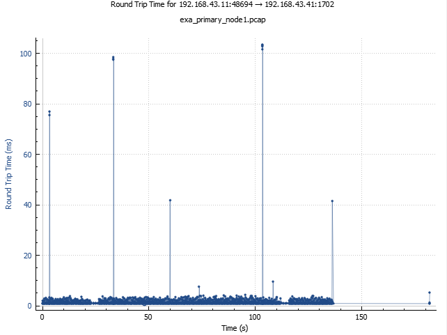
The most striking difference is frequent spikes around 40 ms which are not present on the baseline graph. That’s almost 40 times as much as the normal round-trip time. Also, this matches the size of default value of delayed ACK timeout for some Linux distributions, and checking with ss (socket statistics) utility confirmed that indeed 40 ms was the delayed ACK timeout in this case as well. Finally, when zooming in on a spike one can see that they are not strictly vertical — instead, a quick climb is followed by a linear decay, which means that packets are accumulated somewhere, and then released at the same time.

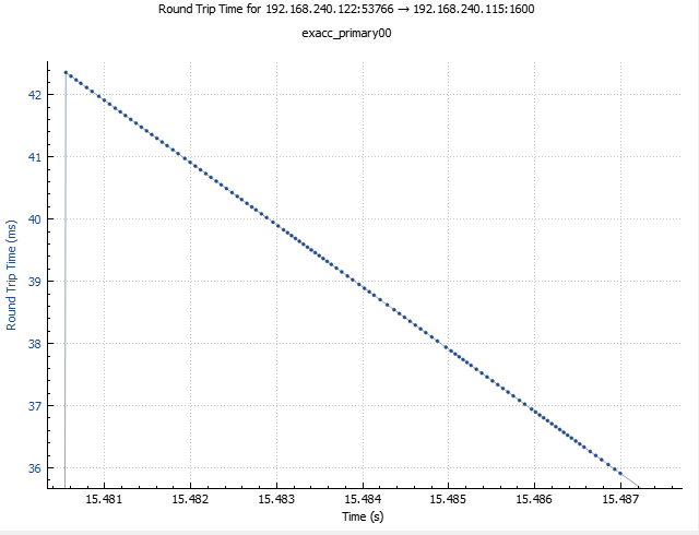
The linear decline does not go all the way to the zero mark, which means that typically, packet accumulation would stop soon after its start, and then for the most part of the timeout no further packets would be accepted, resulting in a gap in the transmission comparable to 40 ms in duration. It’s easy to see, if such gaps are frequent enough, overall impact on the throughput can be devastating, but whether this was the case here, it is difficult to say. 

The reasoning above does not mean that delayed ACKs are always bad, or even that they are always bad for this particular kind of traffic. More likely the harmful effect comes from interacting of this TCP setting with some other, e.g. Nagle algorithm (designed to improve efficiency of TCP by disallowing sending of very small packets in some cases) is known to make a toxic combination with delayed ACK. Of course the simplest way to understand the impact of delayed ACKs would be by disabling them and examining the effect. However, on our Linux distribution such a setting didn’t seem to be available. I used BCC trace.py utility to make sure that Nagle algorithm was, in fact, off (nonagle=1 in tcp_xmit_write calls). 

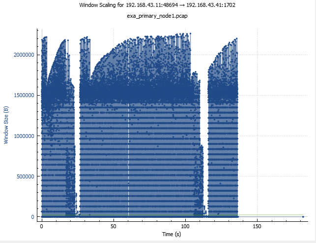
Window scaling graphs are equally interesting. For bytes-in-flight (which estimate the congestion window) the baseline one has all classical features of a normally working  TCP protocol: slow start, quick cubic growth, occasional drops followed by a quick recovery. The size of the congestion window is between 2-3 megabytes which accounts for  excellent transfer rate (if you can send up to 3 MB of data before an ACK is required and RTT is about 1 ms then theoretically you can be sending data at rates up to 3 GB/s).

The same graph for the ExaCC test case looks dramatically different. Only rarely there are bursts reaching values in the neighborhood of 3 MB, but most of the time the amount of data in flight stays in the region of 200,000kB or lower. It’s not likely to have anything to do with the congestion control mechanism as the pattern doesn’t really fit (with congestion control, you expect cubic or similarly shaped growth interspersed with drops due congestion events and rapid recovery), but also because there aren’t many events that could trigger congestion control (such as duplicate ACKs, packet reordering etc.). What about receive window? It’s shown by the green line very close to the x axis. The reason for that is that it’s hasn’t been scaled correctly  due to the 3-way handshake not being present in this packet capture.

To address that, I requested the standby to be bounced while tcpdump capture was still ongoing. That worked well and the new capture file contained the SYN/ACK sequencefrom the  3-way hanshake which carried the necessary flags:

2022-09-01 10:48:21.585355 192.168.240.122                192.168.240.115 TCP 66 57532 → 1600 [SYN] Seq=2622759089 Win=29200 Len=0 MSS=1460 SACK_PERM=1 WS=128

2022-09-01 10:48:21.586560 192.168.240.115 192.168.240.122 TCP 66 1600 → 57532 [SYN, ACK] Seq=3029662401 Ack=2622759090 Win=29200 Len=0 MSS=1460 SACK_PERM=1 WS=128

So we can see that the window scaling (WS) is 128. Another way to obtain this information is with ss utility, but there it is presented differently (as 7, i.e. the binary logarithm of 128). The advantage of having the start of the conversation present in the pcap, however, is that now Wireshark takes the scaling factor into account automatically. This is what the window scaling graph looks for this new capture:

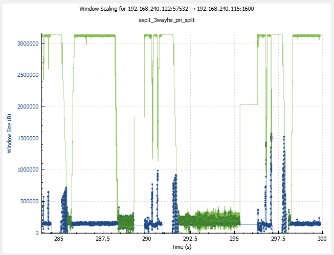
That’s massively better, and we can literally see the outgoing traffic being shaped by the size of the receive window during certain periods. Another curious feature of this graph is that drops in the receive window size are often preceded by a rise in number of bytes-in-flight: so as soon as sender starts transmitting data at a higher rate, the receiver shrinks the receive window as it can’t process incoming data fast enough. So does this mean that the slowness is due to redo apply process on the stanbdy  database not being able to keep up with everything else? Maybe, but let’s not jump to any conclusions just yet. It would seem that an even more interesting peculiarity is that when the receive window recovers to the maximum value, the bytes-in-flight don’t follow and stay flat instead, so perhaps the main limiting factor is yet something else.

With that thought in mind, let’s take a look at the thoughput and segment size graphs. Here again the difference between the ExaCC and the baseline is quite striking.

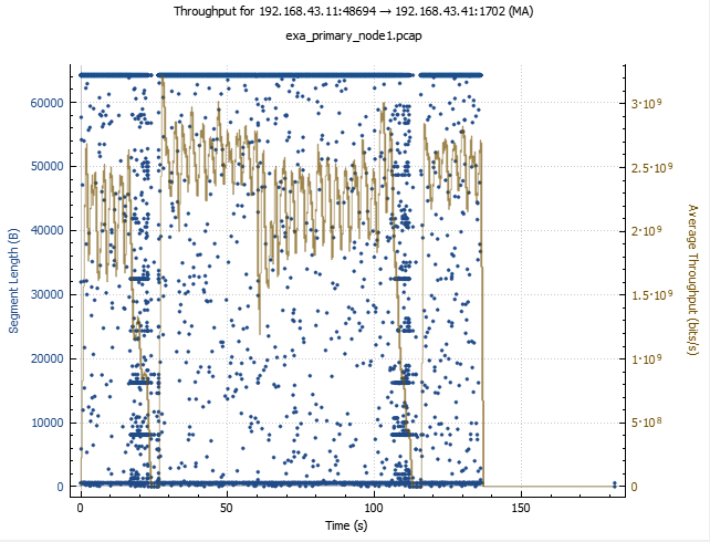
For the baseline, the vast majority of segments are 64kB in size, while for ExaCC is 8kB. Throughput for the baseline stays mostly between 200 and 300 MB/s, as opposed to 50-150 MB/s for the ExaCC. Interestingly enough, some small percentage of segments in the ExaCC capture does have sizes close to 64 kB — and the higher packet size tends to correlated rather well with higher throughput. So could the segment size be the main culprit? Possibly, but nothing is obvious at this point.

Intermediate summary

Since we went through a large volume of information, it would be useful to reiterate the key points established so far:

– Round-trip time (RTT) graph shows that in the ExaCC case, unlike the baseline, there are frequent spikes close to 40 ms. Under zoom one can see that they are followed

by linear decline, as if the packets were accumulated for that duration and then sent all at once. Since 40 ms is the ATO value (delayed ACK timeout), such patterns are

related to delayed ACKs, possibly interacting with some other TCP features. Research shows that a combination of delayed ACKs and Nagle algorithm can be very bad for

the throughput, however, tracing showed that in our case Nagle algorithm was off (nonagle=1 in tcp_xmit_write calls). While transmission gaps that follow the onset of the

linear decline surely hurt the throughput, it’s not immediately clear whether they are frequent enough to account for the reduction in throughput.

– Window scaling doesn’t show any characteristic patterns typical for congestion control limiting the transmission rate. Receive window does show evidence of dropping from the maximum value relatively often, and there are episodes when they reach zero (receiver requests sender to stop the transmission). This looks like evidence of receive window being a factor in limiting the throughput. On the other hand repeating the capture with standby database restarted in the process (to make sure 3-way handshake in present in the capture, providing the value of the scaling factor for the analysis) allowed to get a better picture from which it is clear that receive window is only limiting transmissions during rather short intervals, and probably is not the main problem here. It seems that inability to use all of the receive window when it recovers to the full maximum is probably more important.

– Throughput and segment length graphs show that while most of the segments are 8kB, a small fraction of them are actually bigger (closer to 64 kB), as opposed to mostly

larger segment sizes (64 kB or close) in the baseline capture.  Also, there seems to be some strong positive correlation between segment size and throughput.

To some up, all of this does give some food for though, but nothing is particularly clear, so additional information is required.

Network call tracing

There are several ways to collect additional low-level diagnostics of things happening at the network layer. In this particular case, the simplest one was by using

so called Oracle SQL*Net tracing which is an integral part of their embedded instrumentation framework. One can choose the level of detail for the tracing. Maximum level (16) has a drawback of capturing entire packet contents (inevitably making trace files huge very quickly), so I mostly used the next one, 12.

It should be noted that if vendor’s software does not have such neat built-in instrumentation, there are other ways to do the tracing via dynamic uprobes (e.g. by using trace.py and other utilities in BCC toolkit, perf probe or gdb debugger).

One of the first things that leapt into the eye upon examing the trace file on the sender side was abundance of entries like that:

2022-09-05 21:53:10.550 : nspsend:8156 bytes to transport

which is quite interesting as it tell us that the segmentation all the way down to 8 kB is already happening on the “application” (by which, once again, I mean Oracle Data Guard in this context) layer. That prompted us to repeat the trick with restarting the standby in the middle of a tracing session to capture all connection details, and sure enough, after that was done, we could find things like this in the trace file:

2022-09-05 22:02:10.999 : nsopen:lcl[0]=0xf4ffe9ff, lcl[1]=0x302000, gbl[0]=0xfebf, gbl[1]=0xc01, tdu=4096, sdu=8192

SDU stands for “session data unit” and it’s a parameter that controls the size of a unit of data handled by Oracle’s network layer. By this point in the investigation, it has already drawn our attention a few times, but we were sure it was already set to the maximum allowed value of 64k as prescribed by Oracle documentation. And yet here is clear evidence that it hasn’t worked as we expected!

But at very least we were finally getting something specific, something we could control, and use not only to understand the problem, but also to fix it. One thing that appeared odd, however, was that we clearly saw packets larger than 8kB in the tcpdump — a small fraction of the sample, for sure, but still larger than zero. But according to the SQL*Net trace, 8156 was the maximum packet size there. So if the “application” was sending 8kB packets, how did bigger ones appear in the TCP layer? I didn’t verify it directly, but it seems that the operating system was capable of coalescing small segments into bigger ones. Surely, it didn’t do that all the time, but apparently from time to time there were gaps in transmission (e.g. waiting for a delayed ACK!) that afforded the TCP layer a chance to accumulate a larger packet, thus revealing to us the segmentation issue and its impact on the throughput! It’s quite fascinating how various aspects of the problem interacted here, making it possible for us to discover the root cause.

After some additional research one of DBAs working on this case together with me was able to find an article describing some anomalies about this parameter settings which also suggested some ways around it, and using recommendations from it he was able to achieve the correct SDU size to be reflected in SQL*Net traces. So we re-ran our tests and found that after fixing the SDU issue the performance was… even slightly worse than before.

Just to think that at this point we could have decided “ok, so it’s clearly not the SDU thing, let’s move on to other things” — we could have lost a lot of time this way! Fortunately, with all this instrumentation in place it was straightforward to check the actual packet size, and what we saw was pretty amazing: a stream of packets of 64294 bytes followed by 1302 byte ones… So apparently, when setting the SDU to the maximum allowed value, some small additional overhead caused it go above the 65536 byte limit and get split in two. So we simply tweaked SDU until this weird alignment issue went away (we ended up using 64000 instead of 65535), and finally, the performance issue was solved.

Closing remarks

This article hopefully shows that Wireshark analysis of packet capture can be a powerful tool for troubleshooting a broad class of network-related performance issues on

the application, database, OS, network side or somewhere in between. It probably shouldn’t be the place to start an average investigation: as always with high level of detail, the sheer amount of information can present certain technical challenges. It is also likely to bring to light more anomalies than the one (or ones) that are pointing toward the root cause.

But if initial diagnostics start to point towards the network (in a broad sense), and if high-level network tools such as ss, netstat and/or various benchmarks like qperf don’t give a clear answer, it can be a good way to bring the investigation to a new level. A big advantage of Wireshark is that it allows one to switch comfortably between the “microscopic” and “macroscopic” views of the problem — i.e. you can start by looking at high-level graphs of transmission windows, throughput, round-trip times etc., then you can zoom in on a problem zone, investigate it in high detail, and then click on an individual data point, bringing up the corresponding packet header in the packet header window, and after analyzing that specific sequence of packets go back to looking at other macroscopic graphs etc. This could be a bit more difficult with other low-level tools, e.g. with a SQL*Net trace you may need to parse it to some tabular format before you can extract “macroscopic” information from it (and this extraction would also require additional tools and additional effort).

Successful analysis of packet capture will require some understanding of the network protocol used. In our case it was TCP, one of most common protocols there are. Fortunately, while the full algorithm is quite complex, the fundamentals can be learned in a day or two, and in many cases they will be sufficient. Given the level of maturity of the TCP protocol, one can be tempted to assume that network problems mean that the network itself is somehow “slow”. By the same logic, rather often a quick-and-dirty network test which produces good results can be interpreted as “we checked the network and ruled it out”. Network is an extremely complex system of hardware and software with a lot of knobs to turn, and a lot of things that can go very wrong in there.

Packet analysis is an important tool in network performance analysis, but it’s just one tools out of many, and as always, it’s most efficient when used in combination with others. BCC/BPF framework, for example, contains a huge arsenal of other tools that can be used to supplement (or in some cases replace) packet analysis. One big advantage of it over packet capture is that you don’t need to accumulate huge amounts of diagnostic data — rather, you can analyze things on the fly, do some inline processing of data, and/or use some filters to only look at the information of interest.

Finally, this example hopefully demonstrate vulnerabilities of so-called “checklist” approach (still popular with many engineers). Its essence is identifying a list of “usual suspects” for a given scenario and then going through them ruling them out one by one. In our case we found that the core issue was with the SDU parameter. But we “checked” it early on in the investigation. Just looking at things to see if they have been done “correctly” is an error-prone process. The definition of “correct” can be outdated, confusing or simply plain wrong. In our case, the parameter was set in a way that was prescribed by the official documentation, but as it eventually turned out, that description was, at very least, incomplete. It shouldn’t be very surprising, as e.g. “parameters” often aren’t simple things that are set in one  place in a transparent way and then obediently accepted by the software. Often they are simply “targets” rather than fixed values, or they could be overridden on different levels by other settings, or they can have complex interactions with other parameters etc. So when checking whether a parameter is set correctly just visually confirming the relevant entry in a configuration file may not be enough. Fortunately, various tracing facilities make it possible to also check the value actually used.

Special thanks

to Jonathan Lewis, Ludovico Caldara, Tanel Poder, Ilmar Kerm and many others for their valuable contributions during troubleshooting of this issue, and of course to Stefan Koehler whose article made the solution possible.