Dealing with a global increase in CPU usage

Imagine the following situation: you are supporting an application with many different components and a busy release cycle. One a Monday morning you find that quite a few processes in the database now run slower. Very soon, you find out that the slowdown is due to increased CPU time, but where to move from there? There is no evidence that CPU is too stressed, causing CPU queuing. You cannot isolate the problem to any specific PL/SQL procedure or SQL id, and there seems to be no relationship between affected SQL statements. You also check the changes that went in the last weekend — there are quite a few of them, but none seems to be particularly relevant. So what do you do?

I think that most of us would start by looking at an AWR report, which is not unreasonable. However, one needs to be very careful with

• how the report is to be generated
• what to look for in the report.

The common wisdom is that one should only generate AWR reports for short periods of time. This is simply wrong — the correct approach is to generate them for the duration of the problem. If the problem is there at all times, then the best solution is to look at the entire week so far — the longer the period, the better (because it averages out random fluctuations) — and compare it with a similar period the week before. One can even do an diff report instead of a conventional  one.

The second question — what to look for — is even trickier. When people say “look in the AWR report” they usually mean “look at top wait events”, less often “look at top SQL”. Sometimes load profile gets looked at, or segment level statistics, but in general, an AWR report contains too much information so one usually skims through 1 or 2 most popular sections.

The method that I find much more efficient is looking at instance-level statistics as follows:

1. Calculate weekly averages for the current week and the similar period previous week
2. Keep only those statistics where the change has been considerable (comparable with the size of the performance degradation)
3. Plot the remaining statistics vs time to filter out those with too much jitter.

A further improvement over the method would be to use the averages for the similar periods for all previous weeks within the AWR retention, and calculate their standard deviations to filter out random noise.

The query that I use is shown below:

with a as
(
  select begin_interval_time t, stat_name, value
  from dba_hist_snapshot sn,
       dba_hist_sysstat ss
  where sn.snap_id = ss.snap_id
  and sn.instance_number = 1
  and ss.instance_number = 1
),
b as
(
  select t, t - trunc(t, 'day') time_within_week,  to_char(t, 'ww') week_number, stat_name, value - lag(value) over (partition by stat_name order by t) value
  from a
),
c as
(
  select t, stat_name, trunc(t, 'day') beginning_of_week, time_within_week, value, week_number
  from b
  where time_within_week < systimestamp - trunc(systimestamp, 'day')   and value >= 0
),
d as
(
  select stat_name, week_number, row_number() over (partition by stat_name order by week_number desc) rn, /*rn, */avg(value) value
  from c
  group by stat_name, week_number--, rn
  order by week_number, stat_name
),
f as
(
  select stat_name, avg(value) average_value, stddev(value) stddev_value
  from d
  where rn > 1
  group by stat_name
  order by stat_name
),
g as
(
  select this_week.stat_name, this_week.value current_week_value, prev_weeks.average_value prev_average, prev_weeks.stddev_value prev_stddev
  from f prev_weeks,
       d this_week
  where this_week.rn = 1
  and this_week.stat_name = prev_weeks.stat_name
  and this_week.value > 1000
),
h as
(
  select stat_name,
         trunc(current_week_value) current_week_value,
         trunc(prev_average) prev_weeks_value,
         trunc((current_week_value-prev_average)*100/nullif(prev_average,0)) change_pct,
         trunc(100*prev_stddev/nullif(prev_average,0)) sigma
  from g
)
select *
from h
where abs(change_pct) >= 3*sigma
order by change_pct desc nulls last

As you can see, it only keeps statistics with values over 1000 — this is because you’re typically interested in statistics that are linked to events that occur frequently enough, at least once per minute (on the average). If you think that rare events can be relevant to your problem, you can remove it. Another filter here is abs(change_pct) >= 3*sigma, i.e. only changes less than 3 standard deviations are kept. This way you make sure that you’re looking at metrics that are stable enough, so you know that the change in their values means something.

Let’s look how this approach was applied to a real-life case, where CPU usage went from 20-30% up to 40-50%, and the increase in CPU time cause several unrelated processes in the database to run 20-25% slower.

The query returned following statistics:

• commit cleanout failures: cannot pin (+140%)
• shared hash latch upgrades – wait (+110%)
• redo synch time overhead count ( recursive cpu usage (+48%)
• enqueue waits (+44%)
• CPU used by this session (+38%)
• CPU used when call startded (+37%)
• total number of cf enq holders (+31%)
• bytes via SQL*Net vector to client (+30%)
• redo synch time (+29%)
• redo synch time (usec) (+29%)
• redo synch time overhead (usec) (+27%)
• redo synch time overhead count (+27%).

What of this is really relevant?

First of all, there are commit cleanout feailures. Are they relevant? Probably not, because there is no increase in other commit cleanout statistics, or in reads from UNDO, or in logical I/O.

Next one — “shared hash latch upgrades – wait”. I was unable find the exact description for this statistic, but obiously it has to do with latches, most likely it counts the number of times a latch protecting a hash bucket of the buffer cache was upgraded from shared to exclusive, involving a wait (rather than simple spinning). That sounds interesting, although other latch-related data need to be examined before it can be decided whether or not this is relevant to the problem at hand.

The remaining statistics can be broken into 3 large groups: redo synch related, CPU related and other. “Redo synch” is related to the “log file sync” wait, which indeed was higher than the week before, due to a higher number of commits per unit time. I’ve looked into that and found that a new feed was added that weekend, which increased commits by 25%. The new functionality, however, was relatively self-contained, and since log file sync waits don’t cause CPU usage, I deemed those statistics irrelevant.

CPU statistics were relevant, but they were simply telling me of the problem that I already knew about. I’ve plotted the remaining metrics vs time, using plots like the one shown below.

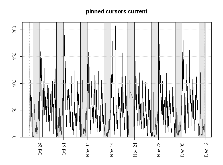
This confirmed that they were irrelevant.

So I took a more detailed look at the latch statistics. I found, that the number of misses on cache buffer chains latch went up dramatically that week:

That confirms that we’ve been looking in the right direction. But how do we fix the problem?

Now that we’ve gathered enough evidence, it’s time to do the theoretical bit. What caused the increase in latching? This particular latch protects a part of the buffer cache, so basically what we are seeing is a sign that we have some “hot blocks” (within the same hash bucket, or buckets) which are being accessed so frequently, that it causes serialization via latching. With that information in mind, I had enough to identify the root cause, as I knew that one of the changes during the last release was about changing a few indexes from reverse to normal. While earlier I discarded this change as irrelevant (as many queries not related to the indexes in question were affected), now it looks different. The very idea of reverse indexes is to spread the access to leaf blocks for indexes on sequence-populated (or monotonously growing for some other reasons) columns. Reversing this change would have obviously caused one or another form of contention for the hot blocks — whether via “buffer busy waits”, or some other enqueues, or via latching.

The change was reversed, and CPU usage went back to normal, and other symptoms disappeared as well.

So let’s reiterate the key aspects of the solution:

1. Look at averages in instance-level statistics before and after the change
2. Be sure to avage over the correct interval: for an application with a weekly cycle (with weekends reserved for maintenance and releases) the natural choice would be a week so far
3. Be sure to compare similar periods, i.e. don’t compare this Monday with previous Friday, if your workload might have distinct periodic patterns (e.g. Mondays could be busier, or less busy, compared to Fridays)
4. Use time plots and related statistics to filter out irrelevant metrics
5. When you’ve narrowed down the list of suspects to just a few, form some reasonable theories linking the increase in observed metrics to the observed increase in CPU usage
6. Obtain additional statistics to confirm your theory, if necessary.

It helps a lot if you can quickly produce high-quality time series plots. R is the ideal tool for this purpose, but you can also use gnuplot or Excel, or some other software.